Rendering multiview images of a scene has been a long standing research area in the field of computer vision. Given multiple images of a scene with varying viewing directions, the task of multiview image synthesis is to generate photorealistic images of the scene with novel views.

Figure 1 : Given multiple input images of a scene with varying viewing directions, a multi view rendering network [1] renders new views of the scene.

Before rendering an image, we first try to represent the scene using an intermediate representation that provides 3D information. Based on the characteristics of these representations they are divided into Explicit, Implicit and Hybrid. In this blog we try to intuitively explain Explicit, Implicit and Hybrid representations as a build up to explaining the method proposed in Efficient Geometry-aware 3D Generative Adversarial Networks [2].

Implicit Representation

The word implicit means “suggested though not directly expressed”. Following this nuance, in implicit representations the 3D information is not definitely expressed. Rather, the 3D scene information is represented using a function. So this forms the ideal recipe for supervised learning where we learn the 3D information by feeding the network with the scene information represented using the camera parameters. Although it seems to be a perfect way to represent a scene, it has its own de-merits.

Before exploring its efficiency, we will look at NeRF (Neural Radiance Fields) [1] as an example for implicit representation. In this work, a deep fully connected network learns the color \(( \begin{bmatrix} R &G &B \end{bmatrix}^T \in \mathbb{R}^3)\) and density \((\sigma \in \mathbb{R})\) information of the scene as a function of the location of a point \(\begin{bmatrix} x &y &z \end{bmatrix}^T\) along a ray and the viewing direction of the scene \(\begin{bmatrix} \theta &\phi \end{bmatrix}^T\). In practice, viewing direction is expressed as a 3D unit vector. The network is learnt by overfitting on a scene i.e. showing images of the same scene captured from different views. During inference, the network regresses the color and density information when queried with a novel camera location and direction.

Figure 2 : A point on the ray along with its viewing direction as shown in (a) is passed through \(F_{\theta}\), which is trained to regress the color and density information as shown in (b). This regressed density and color which vary along the ray (c) is now passed through a volume rendering network to generate an image of the scene which satisfies the underlying viewing direction, \(\begin{bmatrix} \theta &\phi \end{bmatrix}^T\). The entire network comprising of \(F_{\theta}\) and rendering network is trained using the rendering loss which is the squared \(L_2\) norm between the generated image and the the ground truth image (d).

To intuitively understand the output color and density information given by the network, consider a camera ray passing through the scene as shown in Figure 2. The final color information that we see on the image formed is all embedded in this ray. The final color contributed by this ray is the accumulation of all the color surfaces this ray passes through before reaching the camera. And on its way to the camera the ray can pass through different types of transparent, opaque and translucent surfaces. The network essentially tries to trace out the path through which the ray has travelled and this path can be expressed using the color and density information. The output color gives the RGB information of a point \(\begin{bmatrix} x &y &z \end{bmatrix}^T\) on the path while the output density is the probability of a surface being present at that point. Hence, by combining the color and density information we can reconstruct the scene.

Although using this method we get the complete information of the scene, the downside to this approach is its inference time. For querying one input we would need an forward pass through the deep MLP network. And hence explicit representations were introduced to address this issue.

Explicit Representation

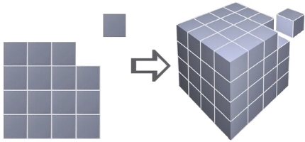
Unlike the implicit representation explained above, in this method we express 3D data using explicitly defined shapes like spheres, cubes, cuboids etc. In this approach, we represent the surface by learning a function \(f\) which maps input images to a 3D grid \(f : \mathbb{R}^2 \rightarrow \mathbb{R}^3\). An example of such a 3D representation is Voxel grid. Voxels are essentially 3D pixels shaped in the form of perfect cubes.

Figure 3 : Difference between a pixel and voxel. For a side of length \(N\), a pixel representation requires \(O\left(N^2\right)\) memory whereas a voxelized representation requires \(O\left(N^3\right)\) memory. Figure 4 : \(A01 – A05\) are examples of how voxel grids of different resolutions model the surface of a car [3].

To understand how a voxel grid represents a 3D scene, consider the car shown in figure 4. If we were to approximate this car’s surface using a 3D voxel grid, in the most basic way we fill up each voxel of the grid with a \(1\) or \(0\) to represent whether or not a part of the car surface is present at that voxel location. Hence using this binary method to populate the voxel grid, we can form a very coarse way to approximate the car’s surface. To also represent finer surface textures, we can increase the number of voxels in the voxel grid there by increasing the number of voxels corresponding to a particular point on the surface.

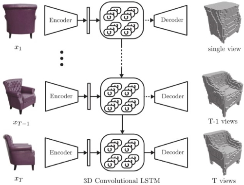
Figure 5 : An overview of a model [4] that takes a sequence of images (or just one image) from arbitrary viewpoints of a scene and generates voxelized 3D reconstruction as output.

In theory, voxel grid is a fast technique for modelling complex surfaces. We can accurately replicate real world objects by employing a proper rendering technique like [4] armed with a very high resolution voxel grid. This approach addresses the inference time problem associated with the implicit representation because in this case we can query the voxel grid in \(O(1)\) time. However this method is inefficient in terms of memory usage as voxel grid requires \(O(N^3)\) memory for a side of length \(N\).

Hybrid Representation

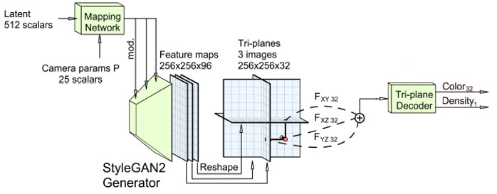
This method takes the best of the two approaches mentioned above and hence is also called explicit-implicit representation. As an example, we will consider Tri-plane hybrid representation [2] which gives color and volume density as the final 3D representation. As shown in figure 6, first, a generator [5] modulated using latent vectors and camera parameters generates explicit features. These features are then projected along three axis-aligned orthogonal feature planes. Second, the projected features are aggregated and fed through a small MLP based light weight decoder generating color and volume density. During inference, a query 3D position \((\mathbf{x} \in \mathbb{R}^3)\) is projected onto each of the three feature planes retrieving the corresponding feature vectors \((F_{xy}, F_{xz}, F_{yz})\).

Figure 6 : Sub network from [2] which generates the tri-plane 3D representation

For a side of length \(N\), the tri-plane representation generates explicit features \(\in \mathbb{R}^{N \times N \times C}\) along each plane, where \(C\) is the number of channels. This implies, tri-plane representation scales with \(O\left(N^2\right)\) while Voxel grid scales with \(O\left(N^3\right)\). As a consequence, tri-plane representation can use higher resolution features and capture greater detail at the cost of a smaller memory. This allows the model to shift bulk of the expressive power of 3D representation to the explicit features while keeping the decoder network small. Thus, the computational cost inccured during inference is much less when compared to implicit representation like NeRF [1].

Summary

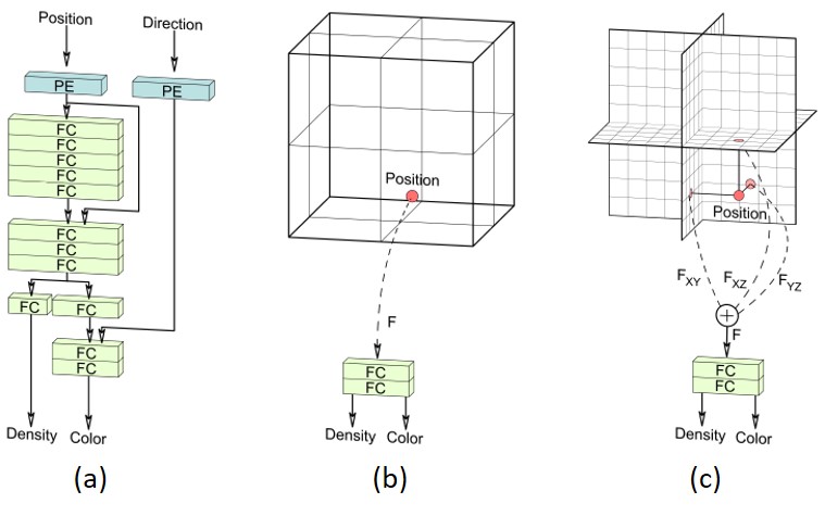
The networks shown in figure 7, summarize the three aproaches mentioned above. The implicit network is accurate but computationally heavy. On the other hand the explicit network is computationally light but memory intensive and the novel hybrid approach finds the middle ground by being light weight and computationally fast.

Figure 7 : Comparison between (a) Implicit, (b) Explicit and (c) Hybrid representations.

References

1. B. Mildenhall, P. P. Srinivasan, M. Tancik, J. T. Barron, R. Ramamoorthi, and R. Ng, “NeRF: Representing Scenes as Neural Radiance Fields for View Synthesis,” in ECCV, 2020.
2. E. R. Chan et al., “Efficient Geometry-aware 3D Generative Adversarial Networks,” in arXiv, 2021.
3. “3D Pixel / Voxel.” .
4. C. B. Choy, D. Xu, J. Y. Gwak, K. Chen, and S. Savarese, “3D-R2N2: A Unified Approach for Single and Multi-view 3D Object Reconstruction,” in Proceedings of the European Conference on Computer Vision (ECCV), 2016.
5. T. Karras, S. Laine, M. Aittala, J. Hellsten, J. Lehtinen, and T. Aila, “Analyzing and Improving the Image Quality of StyleGAN,” in 2020 IEEE/CVF Conference on Computer Vision and Pattern Recognition (CVPR), 2020, pp. 8107–8116.