The term rendering refers to a set of techniques used to generate 2D projections from 3D data of a scene. Most multi view image synthesis pipelines can be divided into 2 blocks. First, scene representation block which constructs a 3D scene representation from multi view images of a given scene. Second, a volume rendering block which is used to generate novel view images of the scene from the learnt 3D scene representation. Depending on the type of representation used in the first block, there exist several volume rendering approaches. In this blog, we explain a radiance field based volume rendering approach.

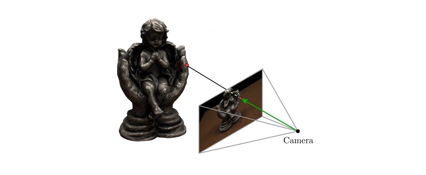
Figure 1 : When queried with a viewing direction, a rendering block generates a 2D projection of the scene [1].

Volume Rendering

A radiance field \(\mathcal{L}\left(\mathbf{x}, \boldsymbol{\theta}\right)\) is a function which maps a point in 3D space \((\mathbf{x})\) and the viewing direction \((\boldsymbol{\theta})\) to a color \(\left(\mathbf{c}\right)\). In practice, the direction \(\boldsymbol{\theta}\) is given by the unit vector \(\mathbf{d}\). So radiance field will be \(\mathcal{L}\left(\mathbf{x}, \mathbf{d}\right)\). Consider points along a ray \(\left(\mathbf{r}\right)\) given by \(\mathbf{x}\left(t\right) = \mathbf{o} + t \mathbf{d}\) where \(\mathbf{o}\) is the origin and \(t \in [t_n, t_f]\) such that \(t_n\) is near bound and \(t_f\) is far bound. The expected color of this ray will be given by

\[C \left(\mathbf{r} \right) = \int_{t_n}^{t_f} \mathbf{c}\left(\mathbf{x}\left(t\right), \mathbf{d} \right) dt\]

In the above equation, we have not considered whether the point is on a particle or not. Intuitively, the expected color of the ray should be influenced more by the colors on the particles. This can be incorporated by weighing color at each point with a term that gives high value if a particle is present and a low value otherwise. We will use volume density \(\sigma\left(\mathbf{x}\right)\) as the weighing term which can be interpreted as the probability of a ray terminating on a particle at \(\mathbf{x}\). The expected color will now be given by

\[\begin{equation} C\left(\mathbf{r}\right) = \int_{t_n}^{t_f} \sigma\left(\mathbf{x}\left(t\right)\right) \mathbf{c}\left(\mathbf{x}\left(t\right), \mathbf{d}\right) dt \end{equation}\]

Once a ray has hit an opaque particle at \(t_i\), it terminates. So points beyond \(t_i\) will not contribute to the expected color of the ray. For this, we will introduce a term known as accumulated transmittance which gives the probability of a ray travelling from \(t_n\) to \(t\) without hitting any particle. It is given by

\[\begin{equation} T\left(t\right) = \text{exp}\left(-\int_{t_n}^t \sigma\left(\mathbf{x}\left(s\right)\right) ds\right) \tag{1} \end{equation}\]

Incorporating all the factors, the expected color of a ray \(\mathbf{r}\) will be given by

\[\begin{equation} C\left(\mathbf{r}\right) = \int_{t_n}^{t_f} T\left(t\right) \sigma\left(\mathbf{x}\left(t\right)\right) \mathbf{c}\left(\mathbf{x}\left(t\right), \mathbf{d}\right) dt \tag{2} \end{equation}\]

Since it is practically not possible to have a continuous set of points, the above integral is numerically estimated using quadrature rule [2] for a discrete set of points \(\{t_i\}_{i=1}^N\). We define \(\delta_i = t_{i+1} - t_i\) as the distance between adjacent samples. The estimated accumulated transmittance \(\hat{T}\) and \(\hat{C}\) are given by

\[\begin{equation} T_i = \text{exp}\left(-\sum_{j=1}^{i-1} \sigma_j \delta_j \right) \tag{3} \end{equation}\] \[\begin{equation} \hat{C}\left(r\right) = \sum_{i=1}^{N} T_i \left(1 - \text{exp}\left( -\sigma_i \delta_i \right) \right) \mathbf{c}_i \tag{4} \end{equation}\]

The above equation can be interpreted as a linear combination of colors along the sampled points on the ray. Thus the expected color can be written as

\[\begin{equation} \hat{C} = \sum\limits_{i=1}^{N} w_i \mathbf{c}_i \tag{5} \label{eq:weighted} \end{equation}\]

where \(w_i\) is the weight given to \(\mathbf{c}_i\) and is given by \(w_i = T_i \left(1 - \text{exp}\left( -\sigma_i \delta_i \right) \right)\). The weight is made up of two terms with the first term taking into account historical information and the second term the current information.

When radiance field gives output in RGB color space i.e. \(\mathbf{c} \in \mathbb{R}^3\) is an RGB vector, the output of volume rendering is the final image. But, when \(\mathbf{c} \in \mathbb{R}^d\) is a feature vector, the output of volume rendering is a feature image. Feature images contain more information that can be used for image space refinement [3]. This allows rendering at lower resolutions and then upsampling to required resolution using convolutional layers. Rendering at lower resolutions helps in faster training and maintaining interactive frame rates.

Sampling points along a ray

The color of each pixel in the generated image is found from the ray terminating at that pixel. Hence to accurately estimate the pixel color, we ideally would need the color information at every point along that ray from \([t_n, t_f]\). Since it is not practically possible to consider every point along the ray, we sample points along it.

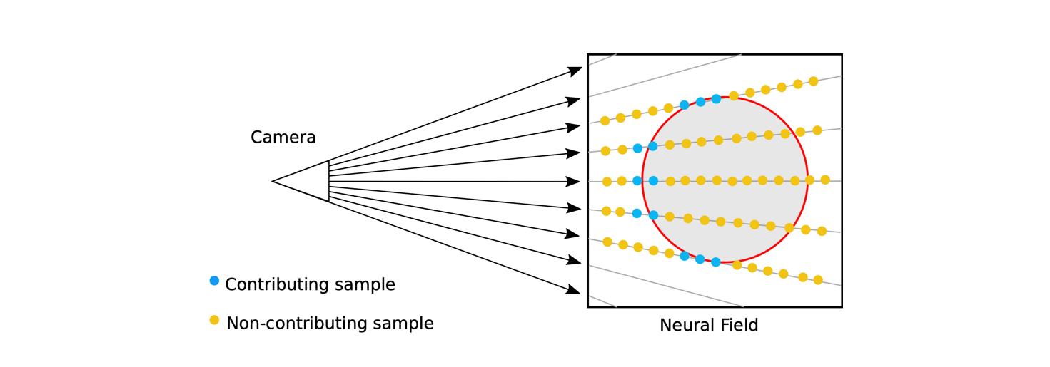
Figure 2 : Uniform sampling of points results in most points not contributing to the expected color of the ray. [4]

The two most commonly used sampling techniques are Stratified sampling and Hierarchical volume sampling or Importance sampling [5]. Consider a ray \(\mathbf{r}\) originating from the point \(\mathbf{o}\). The stratified sampling approach builds upon uniform sampling wherein we take \(N\) equidistant points along the ray. Here, we uniformly divide \(\mathbf{r}\) into \(N\) evenly spaced bins \(\{b_i\}_{i=1}^{N}\) and then draw one sample uniformly at random from each bin. In this approach the number of points sampled will be equal to the number of bins.

\[\begin{equation} t_i \sim U \left[ t_n + \frac{i-1}{N} ( t_f - t_n ), t_n + \frac{i}{N} ( t_f -t_n ) \right] \end{equation}\]

One evident drawback of this approach is that it picks one sample from each bin without considering the contribution of that sample to the final image. This approach also samples from free spaces and occluded regions along the path of \(\mathbf{r}\) that do not contribute to the rendered image. To address this issue a hierarchical sampling approach is used which increases rendering efficiency by allocating samples proportionally to their expected effect on the final rendering.

In Hierarchical / Importance sampling approach, two sets of points are sampled. First, a set of \(N_c\) locations are sampled using stratified sampling and a “coarse” network is evaluated at these locations using equation \(\ref{eq:weighted}\). The expected coarse color \(\hat{C}_c\) of the ray can be formally written as:

\[\hat{C_c} = \sum_{i=1}^{N_c} w_i \mathbf{c}_i\]

The “coarse” output color \(\hat{C}_c\) is refined by re-sampling points along the ray. This “fine” re-sampling is performed by taking into account \(w_i\), which is a direct indication of the contribution of each of the previously sampled \(N_c\) points.

While re-sampling, the task is to have more samples around the points for which \(w_i\) is higher. This is achieved by performing inverse transform sampling.

Inverse transform sampling

Given a uniform distribution \(\mathcal{U}(0,1)\) and a target distribution \(f_X(x)\), inverse transform sampling finds a transformation \(T\) such that, \(T(\mathcal{U}) \sim f_X(x)\).

Figure 3 : Inverse transform sampling is used to find the transformation which converts uniform distribution to an arbitrary target distribution.

If we consider \(F_X(x)\) as the CDF of the target distribution, the relation between \(T\) and \(F_X(x)\) can be found as follows:

\[F_x(x) = P ( X \leq x ) = P ( T ( U ) \leq x ) = P ( U \leq T^{-1}(x) ) = T^{-1}(x)\]

Hence, the required transformation is the inverse of the CDF of the target distribution.

This approach can be employed for re-sampling the points by transforming \(\mathcal{U} \left[ 0 , 1 \right]\) to get the target PDF \(f_X(x)\) which can be obtained by normalizing the weights \(w_i\).

\[f_X(x) = \frac{w_i}{\sum\limits_{j=1}^{N_c} w_j } ~~~~ x \in b_i\]

Hence, sampling \(F_X^{-1}(x)\) will generate points closer to the initial set of samples whose corresponding \(w_i\) was higher. The second set of \(N_f\) locations sampled from this distribution along with the initial \(N_c\) samples are used to evaluate the “fine” network. The final rendered color of the ray can be found by evaluating equation \(\ref{eq:weighted}\) at all \(N_c + N_f\) samples.

Summary

Given a 3D scene representation, the task of a rendering block is to generate 2D projections of the scene. This block estimates the color of each pixel in the output image by sampling points along the ray which terminates at that pixel. This blog explains in detail, a radiance field based volume rendering approach and sampling strategies associated with it.

References

1. M. Niemeyer, L. Mescheder, M. Oechsle, and A. Geiger, “Differentiable Volumetric Rendering: Learning Implicit 3D Representations Without 3D Supervision,” in 2020 IEEE/CVF Conference on Computer Vision and Pattern Recognition (CVPR), 2020, pp. 3501–3512.
2. “Gauss quadrature formula.” Encyclopedia of Mathematics.
3. M. Niemeyer and A. Geiger, “GIRAFFE: Representing Scenes as Compositional Generative Neural Feature Fields,” in 2021 IEEE/CVF Conference on Computer Vision and Pattern Recognition (CVPR), 2021, pp. 11448–11459.
4. M. Piala and R. Clark, “TermiNeRF: Ray Termination Prediction for Efficient Neural Rendering,” in 2021 International Conference on 3D Vision (3DV), 2021, pp. 1106–1114.
5. B. Mildenhall, P. P. Srinivasan, M. Tancik, J. T. Barron, R. Ramamoorthi, and R. Ng, “NeRF: Representing Scenes as Neural Radiance Fields for View Synthesis,” in ECCV, 2020.